5.5 nanoGPT

The simplest, fastest repository for training/finetuning medium-sized GPTs.

Created Date: 2025-08-12

If you're curious about how AI products like ChatGPT work, this tutorial is for you. We'll start from the very beginning, and all you need is a solid grasp of the Python language. Any other concepts will be referenced as we go. Most importantly, we'll be studying the nanoGPT library, an excellent resource for learning how to build large language models from scratch, which was written by the renowned AI educator Andrej Karpathy.

nanoGPT is the simplest, fastest repository for training/finetuning medium-sized GPTs. It is a rewrite of minGPT that prioritizes teeth over education. Still under active development, but currently the file train.py reproduces GPT-2 (124M) on OpenWebText, running on a single 8XA100 40GB node in about 4 days of training. The code itself is plain and readable: train.py is a ~300-line boilerplate training loop and model.py a ~300-line GPT model definition, which can optionally load the GPT-2 weights from OpenAI. That's it.

Figure 1 - The Different Between nanoGPT and ChatGPT

The tutorial is split into two phases. In the first phase, we'll write a character-level generative model from scratch, using Shakespeare's complete works as our training data. This will result in a model that can write in the style of Shakespeare. The second phase involves running a pre-trained GPT model. We won't train it ourselves, as that's too computationally expensive for a personal computer. Instead, we'll download its pre-trained parameters to run inference, and we'll also have the option to finetune it.

5.5.1 Character-Level GPT

If you are not a deep learning professional and you just want to feel the magic and get your feet wet, the fastest way to get started is to train a character-level GPT on the works of Shakespeare.

5.5.1.1 Shakespeare Dataset

William Shakespeare was an English playwright, poet and actor. He is widely regarded as the greatest writer in the English language and the world's pre-eminent dramatist.

The training text is a collection of excerpts from several of Shakespeare's classic plays, mainly including the following works:

• Coriolanus: Accounting for the largest proportion, it presents the complete tragic arc of the protagonist Caius Marcius (later known as Coriolanus) – from a Roman hero to being exiled, eventually allying with former enemies, and finally abandoning his revenge due to his mother's persuasion. It involves class conflicts, personal honor, and power struggles.

• Richard III: It tells the story of Richard III's conspiracies and rule, including his usurpation of the throne, elimination of political opponents, and eventual downfall, demonstrating the desire for power and the distortion of human nature.

• Richard II: Centering on the overthrow of Richard II by Henry Bolingbroke (later Henry IV), it explores the themes of the legitimacy of royal power and betrayal.

Here is a small excerpt from Coriolanus:

First Citizen:
Before we proceed any further, hear me speak.

All:
Speak, speak.

First Citizen:
You are all resolved rather to die than to famish?

All:
Resolved. resolved.

First Citizen:
First, you know Caius Marcius is chief enemy to the people.

All:
We know't, we know't.

File shakespeare_char.py download the input.txt to local data/ directory, and read it in code:

data_dir = os.path.join(os.path.dirname(__file__), "data")
os.makedirs(data_dir, exist_ok=True)
input_file_path = os.path.join(data_dir, "input.txt")

# download the tiny shakespeare dataset
if not os.path.exists(input_file_path):
    with open(input_file_path, "w") as f:
        f.write(requests.get(data_url).text)

with open(input_file_path, "r") as f:
    data = f.read()

print("Length of dataset in characters:", len(data))

Length of dataset in characters: 1115394

Get all the unique characters that occur in this text:

chars = sorted(list(set(data)))
vocab_size = len(chars)
print("All the unique characters:", "".join(chars))
print(f"Vocab size: {vocab_size}")

All the unique characters: 
 !$&',-.3:;?ABCDEFGHIJKLMNOPQRSTUVWXYZabcdefghijklmnopqrstuvwxyz
Vocab size: 65

The vocab chars contains the entire character for our generative model. Predicting the next character means computing the probability of every character in this vocabulary, and then selecting the one with the highest probability to be the predicted output.

Figure 2 - Predict Next Word

# create a mapping from characters to integers
stoi = {ch: i for i, ch in enumerate(chars)}
itos = {i: ch for i, ch in enumerate(chars)}
print(stoi)

{'\n': 0, ' ': 1, '!': 2, '$': 3, '&': 4, "'": 5, ',': 6, '-': 7, '.': 8, '3': 9, ':': 10, ';': 11, '?': 12, 'A': 13, 'B': 14, 'C': 15, 'D': 16, 'E': 17, 'F': 18, 'G': 19, 'H': 20, 'I': 21, 'J': 22, 'K': 23, 'L': 24, 'M': 25, 'N': 26, 'O': 27, 'P': 28, 'Q': 29, 'R': 30, 'S': 31, 'T': 32, 'U': 33, 'V': 34, 'W': 35, 'X': 36, 'Y': 37, 'Z': 38, 'a': 39, 'b': 40, 'c': 41, 'd': 42, 'e': 43, 'f': 44, 'g': 45, 'h': 46, 'i': 47, 'j': 48, 'k': 49, 'l': 50, 'm': 51, 'n': 52, 'o': 53, 'p': 54, 'q': 55, 'r': 56, 's': 57, 't': 58, 'u': 59, 'v': 60, 'w': 61, 'x': 62, 'y': 63, 'z': 64}

Why do we need to tokenize? It's because machines can only process numbers, while words and text are abstractions created by humans. Tokenization is the process of converting these human abstractions into a numerical format that a machine can understand and work with. Therefore, we've defined the encode and decode functions to act as a bridge between humans and machines:

def encode(s):
    # encoder: take a string, output a list of integers
    return [stoi[c] for c in s]

def decode(l):
    # decoder: take a list integers, output a string
    return ''.join([itos[i] for i in l])

Convert the text Hello, World! into tokens. In this case, each character is a token. The encode function maps each character to a unique integer ID. For example, 'H' might become 12, 'e' might become 5, and so on. We can use the decode function to perform the reverse operation: converting a list of numerical tokens back into human-readable text.

sample_text = 'Hello, World!'
print('Tokenize', encode(sample_text))
print('Decode:', decode(encode(sample_text)))

Tokenize [20, 43, 50, 50, 53, 6, 1, 35, 53, 56, 50, 42, 2]
Decode: Hello, World!

Use Python's slicing method to split our data into two categories: a training set (90%) and a validation set (10%). The training set is used to teach the model, while the validation set is used to evaluate its performance.

# create the train and val splits
n = len(data)
train_data = data[:int(n*0.9)]
val_data = data[int(n*0.9):]

# encode both to integers
train_ids = encode(train_data)
val_ids = encode(val_data)
print(f'Train has {len(train_ids)} tokens')
print(f'Val has {len(val_ids)} tokens')

Train has 1003854 tokens
Val has 111540 tokens

Save train_ids and val_ids in this binary format makes them much faster to load later when the training process begins:

# export to bin files
train_ids = numpy.array(train_ids, dtype=numpy.uint16)
val_ids = numpy.array(val_ids, dtype=numpy.uint16)
train_ids.tofile(os.path.join(data_dir, "train.bin"))
val_ids.tofile(os.path.join(data_dir, "val.bin"))

Save the meta information as well, to help us encode/decode later:

meta = {
    "vocab_size": vocab_size,
    "itos": itos,
    "stoi": stoi,
}

with open(os.path.join(data_dir, "meta.pkl"), "wb") as f:
    pickle.dump(meta, f)

5.5.1.2 Model Architecture

This section will be quite long and requires a lot of prerequisite knowledge, such as an understanding of attention mechanisms and the Transformer architecture. If these concepts are new to you, I highly recommend reading my other detailed articles on these topics, as they are crucial for understanding GPT.

• Attention Mechanism

• Attention Is All You Need

• Translate Text with Transformer

Decoder Only

A GPT decoder-only model is a type of Transformer architecture (Figure 4) , as the name suggests, only uses the decoder portion of the original Transformer model. Unlike the original encoder-decoder model, which has separate components for processing the input (encoder) and generating the output (decoder), a decoder-only model combines these two functions into a single unit. This architecture is particularly well-suited for text generation tasks, as it is designed to predict the next word or token in a sequence. ChatGPT and other large language models (LLMs) are prime examples of this architecture.

While removing the encoder, the cross attention in the decoder is also removed. Therefore, the architecture of GPT becomes very simple, as shown below:

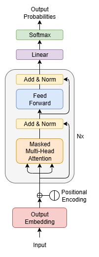
Figure 3 - GPT Architecture

Embedding , softmax , linear layer and Residual network as mentioned in the previous tutorial, the attention module will be covered in the next section. File train.py implements the architecture, let's break this down into a few parts.

Here is a every common multilayer perceptron (MLP) , it's composed mainly of two symmetric torch.nn.Linear :

class MLP(torch.nn.Module):
    def __init__(self, config):
        super().__init__()
        self.c_fc = torch.nn.Linear(config.n_embd, 4 * config.n_embd, bias=config.bias)
        self.gelu = torch.nn.GELU()
        self.c_proj = torch.nn.Linear(
            4 * config.n_embd, config.n_embd, bias=config.bias
        )
        self.dropout = torch.nn.Dropout(config.dropout)

    def forward(self, x):
        x = self.c_fc(x)
        x = self.gelu(x)
        x = self.c_proj(x)
        x = self.dropout(x)
        return x

The Block is the core of GPT , mainly include a CausalSelfAttention and a MLP. Additionally, it includes two residual networks and torch.nn.LayerNorm :

class Block(torch.nn.Module):
    def __init__(self, config):
        super().__init__()
        self.ln_1 = torch.nn.LayerNorm(config.n_embd, bias=config.bias)
        self.attn = CausalSelfAttention(config)
        self.ln_2 = torch.nn.LayerNorm(config.n_embd, bias=config.bias)
        self.mlp = MLP(config)

    def forward(self, x):
        x = x + self.attn(self.ln_1(x))
        x = x + self.mlp(self.ln_2(x))
        return x

Parameters

Before we dive into the deep code details, let's first go over the initial parameters of the system:

@dataclass
class GPTConfig:
    block_size: int = 1024
    # GPT-2 vocab_size of 50257, padded up to nearest multiple of 64 (50304) for efficiency.
    # For our simple character GPT, 128 enough.
    vocab_size: int = (128)
    n_layer: int = 12
    n_head: int = 12
    n_embd: int = 768
    dropout: float = 0.0
    # True: bias in Linears and LayerNorms, like GPT-2. False: a bit better and faster
    bias: bool = (True)

Here are the parameters defined in the GPTConfig class:

• block_size : This is the maximum context length or the number of tokens the model can look back at to make a prediction. A value of 1024 is standard for many models, but it can be adjusted depending on the task and available memory.

• vocab_size : This specifies the size of the vocabulary, which is the total number of unique tokens the model can understand. For the character-level GPT, 128 is sufficient to cover all standard ASCII characters. GPT-2, for example, has a much larger vocabulary of 50,257.

• n_layer : This is the number of transformer blocks (or layers) stacked on top of each other. More layers allow the model to learn more complex patterns but also increase computational cost. A value of 12 is a common choice for smaller models.

• n_head : This is the number of attention heads in the multi-head attention mechanism. Each head can learn different aspects of the input sequence. A value of 12 means the model will split the embedding dimension into 12 parts and apply attention to each part independently.

• n_embd : This is the size of the embedding dimension. It represents the size of the vector used to represent each token in the model. A larger embedding dimension allows for a richer representation of each token's meaning.

• dropout : This is a regularization technique used to prevent overfitting. It sets a fraction of the layer's inputs to zero during training. A dropout rate of 0.0 means no dropout is applied.

• bias : This is a boolean flag that determines whether a bias term is used in the linear layers and LayerNorms. The original GPT-2 used a bias, but setting it to False can sometimes lead to slightly better performance and faster training.

Causal Self Attention

Causal self-attention is a specific type of self-attention mechanism used in transformer models, particularly for tasks like text generation. Unlike standard self-attention, which allows a token to attend to all other tokens in a sequence, causal self-attention enforces a crucial constraint: a token can only attend to the tokens that come before it in the sequence, and not to the tokens that come after.

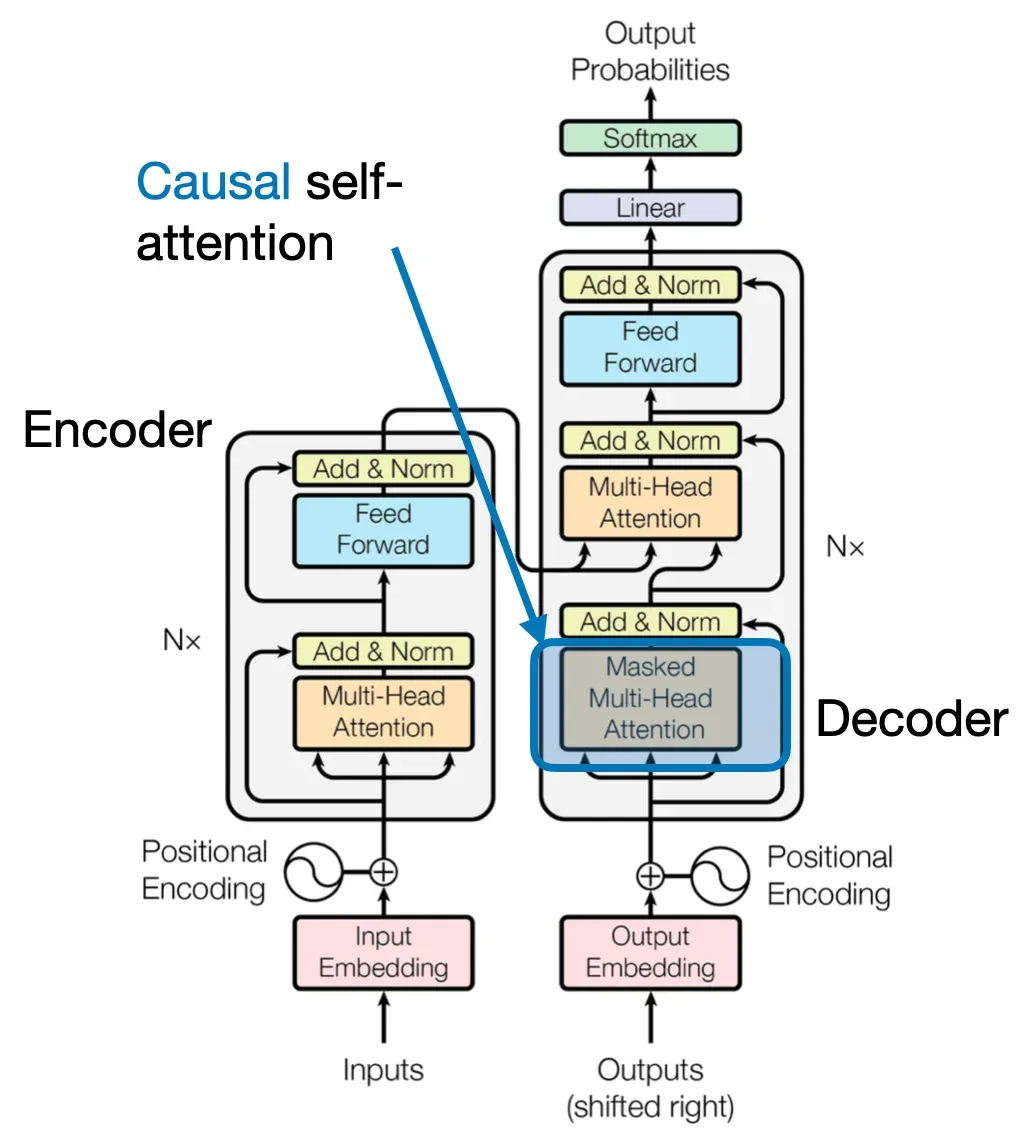
Figure 4 - Casual Self Attention

This "causal" or "masked" approach is essential for autoregressive models like those used in large language models (LLMs) that predict the next word in a sequence. By preventing a model from "cheating" and looking ahead at future words, it ensures that the prediction for each position is based solely on the preceding context.

This is typically implemented by applying a mask to the attention weights, which effectively sets the attention scores for future tokens to negative infinity before applying the softmax function, making their contribution zero.

class CausalSelfAttention(torch.nn.Module):
    def __init__(self, config):
        super().__init__()
        assert config.n_embd % config.n_head == 0
        # key, query, value projections for all heads, but in a batch
        self.c_attn = torch.nn.Linear(
            config.n_embd, 3 * config.n_embd, bias=config.bias
        )
        # output projection
        self.c_proj = torch.nn.Linear(config.n_embd, config.n_embd, bias=config.bias)
        # regularization
        self.attn_dropout = torch.nn.Dropout(config.dropout)
        self.resid_dropout = torch.nn.Dropout(config.dropout)
        self.n_head = config.n_head
        self.n_embd = config.n_embd
        self.dropout = config.dropout
        # flash attention make GPU go brrrrr but support is only in PyTorch >= 2.0
        self.flash = hasattr(torch.nn.functional, "scaled_dot_product_attention")
        if not self.flash:
            print(
                "WARNING: using slow attention. Flash Attention requires PyTorch >= 2.0"
            )
            # causal mask to ensure that attention is only applied to the left in the input sequence
            self.register_buffer(
                "bias",
                torch.tril(torch.ones(config.block_size, config.block_size)).view(
                    1, 1, config.block_size, config.block_size
                ),
            )

    def forward(self, x):
        B, T, C = (
            x.size()
        )  # batch size, sequence length, embedding dimensionality (n_embd)

        # calculate query, key, values for all heads in batch and move head forward to be the batch dim
        q, k, v = self.c_attn(x).split(self.n_embd, dim=2)
        # (B, nh, T, hs)
        k = k.view(B, T, self.n_head, C // self.n_head).transpose(1, 2)
        # (B, nh, T, hs)
        q = q.view(B, T, self.n_head, C // self.n_head).transpose(1, 2)
        # (B, nh, T, hs)
        v = v.view(B, T, self.n_head, C // self.n_head).transpose(1, 2)

        # causal self-attention; Self-attend: (B, nh, T, hs) x (B, nh, hs, T) -> (B, nh, T, T)
        if self.flash:
            # efficient attention using Flash Attention CUDA kernels
            y = torch.nn.functional.scaled_dot_product_attention(
                q,
                k,
                v,
                attn_mask=None,
                dropout_p=self.dropout if self.training else 0,
                is_causal=True,
            )
        else:
            # manual implementation of attention
            att = (q @ k.transpose(-2, -1)) * (1.0 / math.sqrt(k.size(-1)))
            att = att.masked_fill(self.bias[:, :, :T, :T] == 0, float("-inf"))
            att = torch.nn.functional.softmax(att, dim=-1)
            att = self.attn_dropout(att)
            y = att @ v  # (B, nh, T, T) x (B, nh, T, hs) -> (B, nh, T, hs)
        # re-assemble all head outputs side by side
        y = y.transpose(1, 2).contiguous().view(B, T, C)

        # output projection
        y = self.resid_dropout(self.c_proj(y))
        return y

We can understand the code by reading it line by line.

Define a CausalSelfAttention , which is subclass of torch.nn.Module , statement assert ensure the embedding dimension (n_embd) is divisible by the number of attention heads (n_head) :

class CausalSelfAttention(torch.nn.Module):
    def __init__(self, config):
        super().__init__()
        assert config.n_embd % config.n_head == 0

Define two torch.nn.Linear and torch.nn.Dropout layer.

The first linear layer that performs the combined projection for query (Q), key (K) and value (v) vectors. Instead of having three separate linear layers for Q, K, and V, this one layer takes the input embedding (config.n_embd) and projects it to a size that's three times larger (3 * config.n_embd) .

The second linear layer takes the concatenated output from all attention heads (config.n_embd) and projects it back to the original embedding dimension.

# key, query, value projections for all heads, but in a batch
self.c_attn = torch.nn.Linear(config.n_embd, 3 * config.n_embd, bias=config.bias)
# output projection
self.c_proj = torch.nn.Linear(config.n_embd, config.n_embd, bias=config.bias)
# regularization
self.attn_dropout = torch.nn.Dropout(config.dropout)
self.resid_dropout = torch.nn.Dropout(config.dropout)

These is simple, define some variables, because version of PyTorch is great 2.0, so self.flash is True :

self.n_head = config.n_head
self.n_embd = config.n_embd
self.dropout = config.dropout
# flash attention make GPU go brrrrr but support is only in PyTorch >= 2.0
self.flash = hasattr(torch.nn.functional, "scaled_dot_product_attention")
if not self.flash:
    print(
        "WARNING: using slow attention. Flash Attention requires PyTorch >= 2.0"
    )
    # causal mask to ensure that attention is only applied to the left in the input sequence
    self.register_buffer(
        "bias",
        torch.tril(torch.ones(config.block_size, config.block_size)).view(
            1, 1, config.block_size, config.block_size
        ),
    )

The forward function receives an input parameter x , which is a small batch of text. And then unpacks the dimensions of the input tensor x. B is the batch size, T is the sequence length, and C is the embedding dimension (n_embd) :

def forward(self, x):
    # batch size, sequence length, embedding dimensionality (n_embd)
    B, T, C = x.size()

This is where the magic of the combined projection happens. The input x is passed through the c_attn linear layer, and the resulting tensor is split into three equal parts along the last dimension, giving us the query, key, and value tensors.

# calculate query, key, values for all heads in batch and move head forward to be the batch dim
q, k, v = self.c_attn(x).split(self.n_embd, dim=2)

We can write a simple demo to understand above process:

batch_size = 2
seq_length = 3
n_embed = 4

x = torch.randn((batch_size, seq_length, n_embed))
print('Input tensor shape:', x.shape)

c_attn = torch.nn.Linear(n_embed, 3 * n_embed)
result = c_attn(x)
print('Result shape:', result.shape)
q, k, v = result.split(n_embed, dim=2)
print('Query shape:', q.shape)
print('Key shape:', k.shape)
print('Value shape:', v.shape)

Input tensor shape: torch.Size([2, 3, 4])
Result shape: torch.Size([2, 3, 12])
Query shape: torch.Size([2, 3, 4])
Key shape: torch.Size([2, 3, 4])
Value shape: torch.Size([2, 3, 4])

The q, k and v variables is the same shape of x , because we use multi-head, so q, k and v need divide self.n_head parts:

# (B, nh, T, hs)
k = k.view(B, T, self.n_head, C // self.n_head).transpose(1, 2)
# (B, nh, T, hs)
q = q.view(B, T, self.n_head, C // self.n_head).transpose(1, 2)
# (B, nh, T, hs)
v = v.view(B, T, self.n_head, C // self.n_head).transpose(1, 2)

After being divided, the transpose operation will swap the n_head and seq_len dimensions, like the demo shown:

n_head = 2
q = q.view(batch_size, seq_length, n_head, n_embed // n_head).transpose(1, 2)
k = k.view(batch_size, seq_length, n_head, n_embed // n_head).transpose(1, 2)
v = v.view(batch_size, seq_length, n_head, n_embed // n_head).transpose(1, 2)
print('Query divided shape:', q.shape)
print('Key divided shape:', k.shape)
print('Value divied shape:', v.shape)

Query divided shape: torch.Size([2, 2, 3, 2])
Key divided shape: torch.Size([2, 2, 3, 2])
Value divied shape: torch.Size([2, 2, 3, 2])

Function torch.nn.functional.scaled_dot_product_attention calculate the scaled dot product attention, remember we should set is_causal = True :

# causal self-attention; Self-attend: (B, nh, T, hs) x (B, nh, hs, T) -> (B, nh, T, T)
if self.flash:
    # efficient attention using Flash Attention CUDA kernels
    y = torch.nn.functional.scaled_dot_product_attention(
        q,
        k,
        v,
        attn_mask=None,
        dropout_p=self.dropout if self.training else 0,
        is_causal=True,
    )

From a learning perspective, we could also rewrite the scaled_dot_product_attention function. However, in practical applications, it's best to use PyTorch's built-in functions whenever possible.

else:
    # manual implementation of attention
    att = (q @ k.transpose(-2, -1)) * (1.0 / math.sqrt(k.size(-1)))
    att = att.masked_fill(self.bias[:, :, :T, :T] == 0, float("-inf"))
    att = torch.nn.functional.softmax(att, dim=-1)
    att = self.attn_dropout(att)
    y = att @ v  # (B, nh, T, T) x (B, nh, T, hs) -> (B, nh, T, hs)

Transforming the output back to the input's shape:

# re-assemble all head outputs side by side
y = y.transpose(1, 2).contiguous().view(B, T, C)

During the entire attention mechanism process, from the input x to the final output z , we can see that their dimensions do not change. The core reason we use multi-head attention is to help lower the model's loss rate. There's a Chinese proverb that says, "Three humble cobblers are better than one master strategist," which roughly captures the same idea. It means that combining multiple, simpler perspectives can lead to a smarter, more robust solution than relying on a single, complex one.

y = torch.nn.functional.scaled_dot_product_attention(q, k, v, attn_mask=None, is_causal=True)
z = y.transpose(1, 2).contiguous().view(batch_size, seq_length, n_embed)
print('Result of scaled_dot_product_attention:', y.shape)
print('Re-assemble of result:', z.shape)

Result of scaled_dot_product_attention: torch.Size([2, 2, 3, 2])
Re-assemble of result: torch.Size([2, 3, 4])

The c_proj linear layer acts as an output projection for the multi-head attention mechanism. Its primary role is to integrate the different perspectives learned by each of the separate attention heads.

Even though the layer's input and output dimensions are the same, it performs a crucial, learnable linear transformation that fuses all the information from the heads into a single, cohesive representation. This step is essential for creating a meaningful output that is then ready to be used in the subsequent residual connection.

# output projection
y = self.resid_dropout(self.c_proj(y))
return y

GPT Struct

Next, we will assemble the components we've discussed above to create a GPT structure. The following code defines a complete GPT model, which consists of token embeddings, positional encodings, multiple Transformer blocks, and a final classifier head.

class GPT(torch.nn.Module):
    def __init__(self, config):
        super().__init__()
        assert config.vocab_size is not None
        assert config.block_size is not None
        self.config = config

        self.transformer = torch.nn.ModuleDict(
            dict(
                wte=torch.nn.Embedding(config.vocab_size, config.n_embd),
                wpe=torch.nn.Embedding(config.block_size, config.n_embd),
                drop=torch.nn.Dropout(config.dropout),
                h=torch.nn.ModuleList([Block(config) for _ in range(config.n_layer)]),
                ln_f=torch.nn.LayerNorm(config.n_embd, bias=config.bias),
            )
        )
        self.lm_head = torch.nn.Linear(config.n_embd, config.vocab_size, bias=False)

        self.transformer.wte.weight = self.lm_head.weight

        # init all weights
        self.apply(self._init_weights)
        # apply special scaled init to the residual projections, per GPT-2 paper
        for pn, p in self.named_parameters():
            if pn.endswith("c_proj.weight"):
                torch.nn.init.normal_(
                    p, mean=0.0, std=0.02 / math.sqrt(2 * config.n_layer)
                )

        # report number of parameters
        print("number of parameters: %.2fM" % (self.get_num_params() / 1e6,))

    def get_num_params(self, non_embedding=True):
        """
        Return the number of parameters in the model.
        For non-embedding count (default), the position embeddings get subtracted.
        The token embeddings would too, except due to the parameter sharing these
        params are actually used as weights in the final layer, so we include them.
        """
        n_params = sum(p.numel() for p in self.parameters())
        if non_embedding:
            n_params -= self.transformer.wpe.weight.numel()
        return n_params

    def _init_weights(self, module):
        if isinstance(module, torch.nn.Linear):
            torch.nn.init.normal_(module.weight, mean=0.0, std=0.02)
            if module.bias is not None:
                torch.nn.init.zeros_(module.bias)
        elif isinstance(module, torch.nn.Embedding):
            torch.nn.init.normal_(module.weight, mean=0.0, std=0.02)

Instead of using a sine and cosine function for positional encoding, the GPT model uses a learnable torch.nn.Embedding layer because it offers greater expressive power. The wpe = torch.nn.Embedding(config.block_size, config.n_embd) layer creates a lookup table where the model can learn the best vector representation for each position in the sequence, up to block_size .

Just like other deep learning programs, the data is processed by the GPT model to generate a result. This result is then compared with the expected value, and a loss function is used to calculate the difference between the two. In the next section Training , an optimizer will use this loss to update the model's parameters.

def forward(self, idx, targets=None):
    device = idx.device
    b, t = idx.size()
    assert (
        t <= self.config.block_size
    ), f"Cannot forward sequence of length {t}, block size is only {self.config.block_size}"
    pos = torch.arange(0, t, dtype=torch.long, device=device)  # shape (t)

    # forward the GPT model itself
    tok_emb = self.transformer.wte(idx)  # token embeddings of shape (b, t, n_embd)
    pos_emb = self.transformer.wpe(pos)  # position embeddings of shape (t, n_embd)
    x = self.transformer.drop(tok_emb + pos_emb)
    for block in self.transformer.h:
        x = block(x)
    x = self.transformer.ln_f(x)

    if targets is not None:
        # if we are given some desired targets also calculate the loss
        logits = self.lm_head(x)
        loss = torch.nn.functional.cross_entropy(
            logits.view(-1, logits.size(-1)), targets.view(-1), ignore_index=-1
        )
    else:
        # inference-time mini-optimization: only forward the lm_head on the very last position
        logits = self.lm_head(
            x[:, [-1], :]
        )  # note: using list [-1] to preserve the time dim
        loss = None

    return logits, loss

If we pass targets , we are training the model; otherwise, we are predicting (or performing inference). Let's take a detailed look at the loss calculation process in nanGPT.

In training phase, logits.view(-1, logits.size(-1)) reshapes the model's output. The logits tensor initially has a shape of (batch_size, sequence_length, vocab_size). However, the cross_entropy function expects its input to be a 2D tensor, where each row corresponds to a single sample and each column is a class score.

The targets tensor starts with a shape of (batch_size, sequence_length) , holding the true token ID for each position. targets.view(-1) prepares the ground truth labels to match the reshaped logits.

The nanGPT codebase uses a target value of -1 for any token that should be ignored during loss calculation. This typically includes padding tokens at the end of sequences and the very first token, as there's no preceding token to predict it from.

For more information, we can look at the torch.nn.functional.cross_entropy documentation.

5.5.1.3 Training

It's time to training character GPT, to reduce complexity, parameters are not read from the command line. First, execute the shakespeare_char.py file, then executing the train.py file will start the training process.

The implementation in file train.py

def get_batch(split="train"):
    if split == "train":
        data = numpy.memmap(
            os.path.join(data_dir, "train.bin"), dtype=numpy.uint16, mode="r"
        )
    else:
        data = numpy.memmap(
            os.path.join(data_dir, "val.bin"), dtype=numpy.uint16, mode="r"
        )

    ix = torch.randint(len(data) - block_size, (batch_size,))
    x = torch.stack(
        [torch.from_numpy((data[i : i + block_size]).astype(numpy.int64)) for i in ix]
    )
    y = torch.stack(
        [
            torch.from_numpy((data[i + 1 : i + 1 + block_size]).astype(numpy.int64))
            for i in ix
        ]
    )

    if device == "cuda":
        # pin arrays x,y, which allows us to move them to GPU asynchronously (non_blocking=True)
        x, y = x.pin_memory().to(device, non_blocking=True), y.pin_memory().to(
            device, non_blocking=True
        )
    else:
        x, y = x.to(device), y.to(device)
    return x, y

# helps estimate an arbitrarily accurate loss over either split using many batches
@torch.no_grad()
def estimate_loss(batch=200):
    out = {}
    model.eval()
    for split in ["train", "val"]:
        losses = torch.zeros(batch)
        for k in range(batch):
            X, Y = get_batch(split)
            with ctx:
                logits, loss = model(X, Y)
            losses[k] = loss.item()
        out[split] = losses.mean()
    model.train()
    return out

5.5.1.4 Inference

sample.py

5.5.2 Reproducing GPT-2

In February 14, 2019, OpenAI release GPT-2, it was trained simply to predict the next word in 40GB of Internet text. GPT‑2 is a large transformer⁠(opens in a new window)-based language model with 1.5 billion parameters, trained on a dataset of 8 million web pages. GPT‑2 is trained with a simple objective: predict the next word, given all of the previous words within some text. The diversity of the dataset causes this simple goal to contain naturally occurring demonstrations of many tasks across diverse domains. GPT‑2 is a direct scale-up of GPT, with more than 10X the parameters and trained on more than 10X the amount of data.

You can read their paper Language Models are Unsupervised Multitask Learners for more information.

5.5.3 Finetuning

5.5.4 Summary