3.3 ResNet
Deep Residual Learning for Image Recognition
Created Date: 2025-06-22
Deeper neural networks are more difficult to train. We present a residual learning framework to ease the training of networks that are substantially deeper than those used previously. We explicitly reformulate the layers as learning residual functions with reference to the layer inputs, instead of learning unreferenced functions. We provide comprehensive empirical evidence showing that these residual networks are easier to optimize, and can gain accuracy from considerably increased depth. On the ImageNet dataset we evaluate residual nets with a depth of up to 152 layers - \(8 \times\) deeper than VGG nets but still having lower complexity. An ensemble of these residual nets achieves 3.57% error on the ImageNet test set. This result won the 1st place on the ILSVRC 2015 classification task. We also present analysis on CIFAR-10 with 100 and 1000 layers.
The depth of representations is of central importance for many visual recognition tasks. Solely due to our extremely deep representations, we obtain a 28% relative improvement on the COCO object detection dataset. Deep residual nets are foundations of our submissions to ILSVRC & COCO 2015 competitions, where we also won the 1st places on the tasks of ImageNet detection, ImageNet localization, COCO detection, and COCO segmentation.
3.3.1 Introduction
Deep convolutional neural networks have led to a series of breakthroughs for image classification. Deep networks naturally integrate low/mid/high-level features and classifiers in an end-to-end multi-layer fashion, and the "levels" of features can be enriched by the number of stacked layers (depth).
Recent evidence reveals that network depth is of crucial importance, and the leading results on the challenging ImageNet dataset all exploit "very deep" models, with a depth of sixteen to thirty. Many other non-trivial visual recognition tasks have also greatly benefited from very deep models.
Driven by the significance of depth, a question arises: Is learning better networks as easy as stacking more layers? An obstacle to answering this question was the notorious problem of vanishing/exploding gradients, which hamper convergence from the beginning. This problem, however, has been largely addressed by normalized initialization and intermediate normalization layers, which enable networks with tens of layers to start converging for stochastic gradient descent (SGD) with backpropagation.
When deeper networks are able to start converging, a degradation problem has been exposed: with the network depth increasing, accuracy gets saturated (which might be unsurprising) and then degrades rapidly. Unexpectedly, such degradation is not caused by overfitting, and adding more layers to a suitably deep model leads to higher training error, as reported in and thoroughly verified by our experiments.
The degradation (of training accuracy) indicates that not all systems are similarly easy to optimize. Let us consider a shallower architecture and its deeper counterpart that adds more layers onto it. There exists a solution by construction to the deeper model: the added layers are identity mapping, and the other layers are copied from the learned shallower model.
The existence of this constructed solution indicates that a deeper model should produce no higher training error than its shallower counterpart. But experiments show that our current solvers on hand are unable to find solutions that are comparably good or better than the constructed solution (or unable to do so in feasible time).
In this paper, we address the degradation problem by introducing a deep residual learning framework. Instead of hoping each few stacked layers directly fit a desired underlying mapping, we explicitly let these layers fit a residual mapping.
Formally, denoting the desired underlying mapping as \(\mathcal{H}(x)\), we let the stacked nonlinear layers fit another mapping of \(\mathcal{F}(x) := \mathcal{H}(x) - x\). The original mapping is recast into \(\mathcal{F}(x) + x\).
We hypothesize that it is easier to optimize the residual mapping than to optimize the original, unreferenced mapping. To the extreme, if an identity mapping were optimal, it would be easier to push the residual to zero than to fit an identity mapping by a stack of nonlinear layers.
The formulation of \(\mathcal{F}(x) + x\) can be realized by feedforward neural networks with "shortcut connections". Shortcut connections are those skipping one or more layers.
In our case, the shortcut connections simply perform identity mapping, and their outputs are added to the outputs of the stacked layers (Fig. 1). Identity shortcut connections add neither extra parameter nor computational complexity. The entire network can still be trained end-to-end by SGD with backpropagation, and can be easily implemented using common libraries without modifying the solvers.
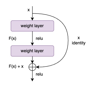
Figure 1 - Residual Learning: a Building Block
We present comprehensive experiments on ImageNet to show the degradation problem and evaluate our method. We show that:
Our extremely deep residual nets are easy to optimize, but the counterpart "plain" nets (that simply stack layers) exhibit higher training error when the depth increases;
Our deep residual nets can easily enjoy accuracy gains from greatly increased depth, producing results substantially better than previous networks.
Similar phenomena are also shown on the CIFAR-10 set, suggesting that the optimization difficulties and the effects of our method are not just akin to a particular dataset. We present successfully trained models on this dataset with over 100 layers, and explore models with over 1000 layers.
On the ImageNet classification dataset, we obtain excellent results by extremely deep residual nets. Our 152 layer residual net is the deepest network ever presented on ImageNet, while still having lower complexity than VGG nets. Our ensemble has 3.57% top-5 error on the ImageNet test set, and won the 1st place in the ILSVRC 2015 classification competition.
The extremely deep representations also have excellent generalization performance on other recognition tasks, and lead us to further win the 1st places on: ImageNet detection, ImageNet localization, COCO detection, and COCO segmentation in ILSVRC & COCO 2015 competitions. This strong evidence shows that the residual learning principle is generic, and we expect that it is applicable in other vision and non-vision problems.
3.3.2 Related Work
In this section, we will introduce the related work of residual learning, including residual representations and shortcut connections.
You don't need to understand too much, because residual learning is a very simple mechanism.
Residual Representations
In image recognition, VLAD is a representation that encodes by the residual vectors with respect to a dictionary, and Fisher Vector can be formulated as a probabilistic version of VLAD. Both of them are powerful shallow representations for image retrieval and classification. For vector quantization, encoding residual vectors is shown to be more effective than encoding original vectors.
In low-level vision and computer graphics, for solving Partial Differential Equations (PDEs), the widely used Multigrid method reformulates the system as subproblems at multiple scales, where each subproblem is responsible for the residual solution between a coarser and a finer scale.
An alternative to Multigrid is hierarchical basis preconditioning, which relies on variables that represent residual vectors between two scales. It has been shown that these solvers converge much faster than standard solvers that are unaware of the residual nature of the solutions. These methods suggest that a good reformulation or preconditioning can simplify the optimization.
Shortcut Connections
Practices and theories that lead to shortcut connections have been studied for a long time. An early practice of training multi-layer perceptrons (MLPs) is to add a linear layer connected from the network input to the output. A few intermediate layers are directly connected to auxiliary classifiers for addressing vanishing/exploding gradients. The papers propose methods for centering layer responses, gradients, and propagated errors, implemented by shortcut connections. An "inception" layer is composed of a shortcut branch and a few deeper branches.
Concurrent with our work, "highway networks" present shortcut connections with gating functions. These gates are data-dependent and have parameters, in contrast to our identity shortcuts that are parameter-free. When a gated shortcut is "closed" (approaching zero), the layers in highway networks represent non-residual functions. On the contrary, our formulation always learns residual functions; our identity shortcuts are never closed, and all information is always passed through, with additional residual functions to be learned. In addition, highway networks have not demonstrated accuracy gains with extremely increased depth (e.g., over 100 layers).
3.3.3 Deep Residual Learning
In this section, we will introduce the deep residual learning framework, which is the core of ResNet. We will explain what residual learning is, how to implement it with code, and how to apply it to different network architectures.
3.3.3.1 Residual Learning
Let us consider \(\mathcal{H}(x)\) as an underlying mapping to be fit by a few stacked layers (not necessarily the entire net), with \(x\) denoting the inputs to the first of these layers. If one hypothesizes that multiple nonlinear layers can asymptotically approximate complicated functions, then it is equivalent to hypothesize that they can asymptotically approximate the residual functions, i.e., \(\mathcal{H}(x) - x\) (assuming that the input and output are of the same dimensions).
So rather than expect stacked layers to approximate \(\mathcal{H}\), we explicitly let these layers approximate a residual function \(\mathcal{F}(x) := \mathcal{H}(x) - x\). The original function thus becomes \(\mathcal{F}(x) +x\). Although both forms should be able to asymptotically approximate the desired functions (as hypothesized), the ease of learning might be different.
This reformulation is motivated by the counterintuitive phenomena about the degradation problem. As we discussed in the introduction, if the added layers can be constructed as identity mappings, a deeper model should have training error no greater than its shallower counterpart.
The degradation problem suggests that the solvers might have difficulties in approximating identity mappings by multiple nonlinear layers. With the residual learning reformulation, if identity mappings are optimal, the solvers may simply drive the weights of the multiple nonlinear layers toward zero to approach identity mappings.
In real cases, it is unlikely that identity mappings are optimal, but our reformulation may help to precondition the problem. If the optimal function is closer to an identity mapping than to a zero mapping, it should be easier for the solver to find the perturbations with reference to an identity mapping, than to learn the function as a new one. We show by experiments that the learned residual functions ingeneral have small responses, suggesting that identity mappings provide reasonable preconditioning.
3.3.3.2 Identity Mapping by Shortcuts
We adopt residual learning to every few stacked layers. A building block is shown in (Fig. 1). Formally, in this paper we consider a building block defined as:
Here \(x\) and \(y\) are the input and output vectors of the layers considered. The function \(\mathcal{F}(x, \{W_i\})\) represents the residual mapping to be learned. For the example in (Fig. 1) that has two layers, \(\mathcal{F} = W_2 \cdot \sigma(W_1 x)\) in which \(\sigma\) denotes ReLU and the biases are omitted for simplifying notations. The operation \(\mathcal{F} +x\) is performed by a shortcut connection and element-wise addition. We adopt the second nonlinearity after the addition (i.e., \(\sigma(y)\), see Fig. 1).
The shortcut connections introduce neither extra parameter nor computation complexity. This is not only attractive in practice but also important in our comparisons between plain and residual networks.
We can fairly compare plain/residual networks that simultaneously have the same number of parameters, depth, width, and computational cost (except for the negligible element-wise addition).
The dimensions of \(x\) and \(\mathcal{F}\) must be equal in above equation. If this is not the case (e.g., when changing the input/output channels), we can perform a linear projection \(W_s\) by the shortcut connections to match the dimensions:
We can also use a square matrix \(W_s\) in above equation. But we will show by experiments that the identity mapping is sufficient for addressing the degradation problem and is economical, and thus \(W_s\) is only used when matching dimensions.
The form of the residual function \(\mathcal{F}\) is flexible. Experiments in this paper involve a function \(\mathcal{F}\) that has two or three layers (Fig. 2), while more layers are possible.
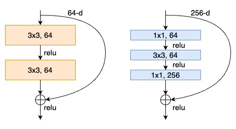
Figure 2 - Residual Function
We also note that although the above notations are about fully-connected layers for simplicity, they are applicable to convolutional layers. The function \(\mathcal{F}(x, {W_i})\) can represent multiple convolutional layers. The element-wise addition is performed on two feature maps, channel by channel.
3.3.3.3 Network Architectures
We have tested various plain/residual nets, and have observed consistent phenomena. To provide instances for discussion, we describe two models for ImageNet as follows.
Plain Network
Our plain baselines (Fig. 3, middle) are mainly inspired by the philosophy of VGG nets (Fig. 3, left). The convolutional layers mostly have \(3 \times 3\) filters and follow two simple design rules:
For the same output feature map size, the layers have the same number of filters;
If the feature map size is halved, the number of filters is doubled so as to preserve the time complexity per layer.
We perform downsampling directly by convolutional layers that have a stride of 2. The network ends with a global average pooling layer and a 1000-way fully-connected layer with softmax. The total number of weighted layers is 34 in Fig. 3 (middle).
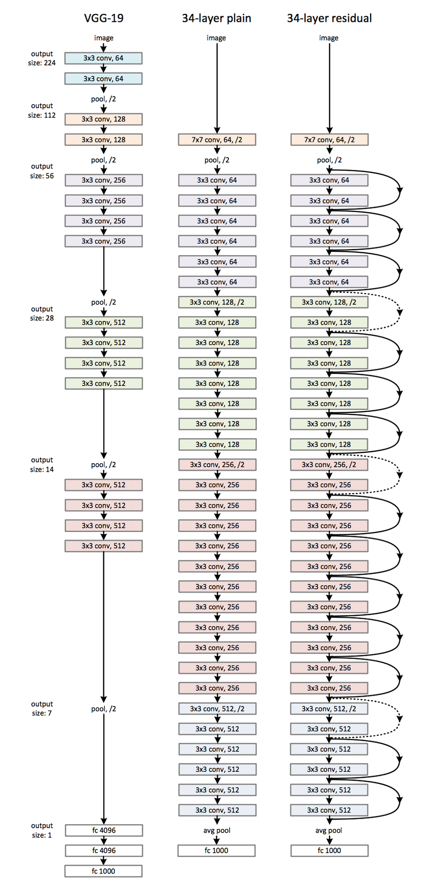
Figure 3 - Example Network Architectures for ImageNet
It is worth noticing that our model has fewer filters and lower complexity than VGG nets. Our 34-layer baseline has 3.6 billion FLOPs (multiply-adds), which is only 18% of VGG-19 (19.6 billion FLOPs).
Residual Network
Based on the above plain network, we insert shortcut connections (Fig. 3, right) which turn the network into its counterpart residual version. The identity shortcuts equation can be directly used when the input and output are of the same dimensions (solid line shortcuts in Fig. 3).
When the dimensions increase (dotted line shortcuts in Fig. 3), we consider two options:
The shortcut still performs identity mapping, with extra zero entries padded for increasing dimensions. This option introduces no extra parameter;
The projection shortcut equation is used to match dimensions (done by 1×1 convolutions). For both options, when the shortcuts go across feature maps of two sizes, they are performed with a stride of 2.