2.2 基础文本分类
构建二元分类器模型来对 IMDB 数据集(文本)执行情绪分析!
创建日期: 2022-07-22
本教程演示了从磁盘中读取纯文本进行文本分类,我们会训练一个 二元分类器 (Binary Classifier) 对 IMDB 电影评论数据集进行情绪分析,代码在 basic_text_classify.py 文件里。
2.2.1 数据处理
本教程训练了一个情绪分析模型,将电影评论分为正面或负面,这是一个二元分类的示例,是一种重要且广泛适用的机器学习模型。
将使用包含 50000 条电影评论文本的大型数据集,其中 25000 条用于训练,25000 用于测试。
2.2.1.1 IMDB 数据集
让我们下载并提取数据集,然后探索目录结构。
url = "https://ai.stanford.edu/~amaas/data/sentiment/aclImdb_v1.tar.gz"
dataset = keras.utils.get_file('aclImdb_v1', url,
                untar=True,
                cache_subdir='')
dataset_dir = os.path.join(os.path.dirname(dataset), 'aclImdb_v1/aclImdb')
print(os.listdir(dataset_dir))
train_dir = os.path.join(dataset_dir, 'train')
print(os.listdir(train_dir))
['imdb.vocab', 'imdbEr.txt', 'README', 'test', 'train'] ['labeledBow.feat', 'neg', 'pos', 'unsup', 'unsupBow.feat', 'urls_neg.txt', 'urls_pos.txt', 'urls_unsup.txt']
train/pos 和 train/neg 包含许多文本文件,每个文件都是一篇电影评论,我们来看看其中一个:
sample_file = os.path.join(train_dir, 'pos/1181_9.txt')
with open(sample_file) as f:
    print(f.read())
Rachel Griffiths writes and directs this award winning short film. A heartwarming story about coping with grief and cherishing the memory of those we've loved and lost. Although, only 15 minutes long, Griffiths manages to capture so much emotion and truth onto film in the short space of time. Bud Tingwell gives a touching performance as Will, a widower struggling to cope with his wife's death. Will is confronted by the harsh reality of loneliness and helplessness as he proceeds to take care of Ruth's pet cow, Tulip. The film displays the grief and responsibility one feels for those they have loved and lost. Good cinematography, great direction, and superbly acted. It will bring tears to all those who have lost a loved one, and survived.
2.2.1.2 加载数据集
接下来我们会从磁盘中加载数据,并处理成合适的格式用于训练。使用 text_dataset_from_directory 函数,它期望下面形式的目录:
main_directory/
...class_a/
......a_text_1.txt
......a_text_2.txt
...class_b/
......b_text_1.txt
......b_text_2.txt
要准备用于二元分类的数据集,我们需要磁盘上有两个文件夹,分别对应于 class_a 和 class_b 。这些将是正面和负面的电影评论,可以在 aclImdb/train/pos 和 aclImdb/train/neg 中找到。由于 IMDB 数据集包含其它文件夹,因此需要将它们删除:
remove_dir = os.path.join(train_dir, 'unsup')
shutil.rmtree(remove_dir)
使用 text_dataset_from_directory 函数创建一个 tf.data.Dataset 类型,tf.data 是一个用于处理数据的强大工具集合。
在运行机器学习实验时,最佳做法是将数据集分为三个部分:训练、验证和测试。
IMDB 数据集已分为训练集和测试集,但缺少验证集。让我们设置 validation_split 参数,以 80:20 的比例分割训练数据,创建一个验证集:
BATCH_SIZE = 32
seed = 42
raw_train_ds = keras.utils.text_dataset_from_directory(
    train_dir,
    batch_size=BATCH_SIZE,
    validation_split=0.2,
    subset='training',
    seed=seed)
Found 25000 files belonging to 2 classes. Using 20000 files for training.
如上所示,训练文件夹中有 25000 个示例,将使用其中的 80%(即 20000 个)进行训练。我们可以迭代数据集并打印一些示例,如下所示:
for text_batch, label_batch in raw_train_ds.take(1):
    for i in range(3):
        print('Review:', text_batch.numpy()[i])
        print('Label:', label_batch.numpy()[i])
Review: b'"Pandemonium" is a horror movie spoof that comes off more stupid than funny. Believe me when I tell you, I love comedies. Especially comedy spoofs. "Airplane", "The Naked Gun" trilogy, "Blazing Saddles", "High Anxiety", and "Spaceballs" are some of my favorite comedies that spoof a particular genre. "Pandemonium" is not up there with those films. Most of the scenes in this movie had me sitting there in stunned silence because the movie wasn\'t all that funny. There are a few laughs in the film, but when you watch a comedy, you expect to laugh a lot more than a few times and that\'s all this film has going for it. Geez, "Scream" had more laughs than this film and that was more of a horror film. How bizarre is that?
*1/2 (out of four)' Label: 0 Review: b"David Mamet is a very interesting and a very un-equal director. His first movie 'House of Games' was the one I liked best, and it set a series of films with characters whose perspective of life changes as they get into complicated situations, and so does the perspective of the viewer.
So is 'Homicide' which from the title tries to set the mind of the viewer to the usual crime drama. The principal characters are two cops, one Jewish and one Irish who deal with a racially charged area. The murder of an old Jewish shop owner who proves to be an ancient veteran of the Israeli Independence war triggers the Jewish identity in the mind and heart of the Jewish detective.
This is were the flaws of the film are the more obvious. The process of awakening is theatrical and hard to believe, the group of Jewish militants is operatic, and the way the detective eventually walks to the final violent confrontation is pathetic. The end of the film itself is Mamet-like smart, but disappoints from a human emotional perspective.
Joe Mantegna and William Macy give strong performances, but the flaws of the story are too evident to be easily compensated." Label: 0 Review: b'Great documentary about the lives of NY firefighters during the worst terrorist attack of all time.. That reason alone is why this should be a must see collectors item.. What shocked me was not only the attacks, but the"High Fat Diet" and physical appearance of some of these firefighters. I think a lot of Doctors would agree with me that,in the physical shape they were in, some of these firefighters would NOT of made it to the 79th floor carrying over 60 lbs of gear. Having said that i now have a greater respect for firefighters and i realize becoming a firefighter is a life altering job. The French have a history of making great documentary\'s and that is what this is, a Great Documentary.....' Label: 1
注:文本里的 br 标签在 HTML 里面被解释成为空行。
标签为 0 或 1,查看 class_names 属性确定正面评论对应 1,负面评论对应 0:
print('Label 0 corresponds to', raw_train_ds.class_names[0])
print('Label 1 corresponds to', raw_train_ds.class_names[1])
Label 0 corresponds to neg Label 1 corresponds to pos
接下来,我们将创建验证和测试数据集,使用训练集中剩余的 5000 条评论进行验证:
raw_val_ds = keras.utils.text_dataset_from_directory(
    train_dir,
    batch_size=BATCH_SIZE,
    validation_split=0.2,
    subset='validation',
    seed=seed)
Label 0 corresponds to neg Label 1 corresponds to pos
注:当使用 validation_split 和 subset 时,需要指定一个随机种子,或者传递 shuffle=False ,避免验证集和训练集分割的时候有交叉。
Found 25000 files belonging to 2 classes.
Using 5000 files for validation.
raw_test_ds = keras.utils.text_dataset_from_directory(
    test_dir,
    batch_size=BATCH_SIZE)
Found 25000 files belonging to 2 classes.
2.2.1.3 预处理
接下来,我们需要使用 keras.layers.TextVectorization 层 标准化 (Standardize) 、标记化 (Tokenize) 和 向量化 (Vectorize) 数据集
标准化是指对文本进行预处理,通常是为了删除标点符号或 HTML 元素以简化数据集。标记化是指将字符串拆分未标记(例如通过按空格拆分将句子拆分未单个单词)。矢量化是指将标记转换未数字,以便可以将它们输入到神经网络中。所有这些任务都可以通过 keras.layers.TextVectorization 层来完成。
正如我们在上面看到的,评论包含各种 HTML 标签,例如 br 。这些标签不会被 TextVectorization 层中的默认标准化器删除(默认情况下,它将文本转换为小写并删除标点符号,但是不会删除 HTML)。我们将自定义一个标准化函数来删除 HTML:
def custom_standardization(input_data):
    lowercase = tf.strings.lower(input_data)
    stripped_html = tf.strings.regex_replace(lowercase, '<br />', ' ')
    return tf.strings.regex_replace(stripped_html,
                                    '[%s]' % re.escape(string.punctuation),
                                    '')
创建一个 TextVectorization 层,我们将使用此层来标准化、标记化和矢量化数据,将 output_mode 设置为 int ,为每个标记创建唯一的整数索引。
请注意我们使用的是默认拆分函数和上面自定义的标准化函数。我们还需要为模型定义一些常量,例如句子的最大长度 sequence_length,这将导致将序列填充或截断为精确的 sequence_length 值:
max_features = 10000
sequence_length = 250
vectorize_layer = keras.layers.TextVectorization(
    standardize=custom_standardization,
    max_tokens=max_features,
    output_mode='int',
    output_sequence_length=sequence_length)
接下来我们调用 adapt 将预处理层的状态与数据集相匹配,这将导致模型构建字符串到整数的索引:
# Make a text-only dataset (without labels), then call adapt.
train_text = raw_train_ds.map(lambda x, y: x)
vectorize_layer.adapt(train_text)
注:调用 adapt 时仅使用训练数据非常重要(使用测试集会泄露信息)。
让我们创建一个函数来查看使用该层预处理一些数据的结果:
def vectorize_text(text, label):
    text = tf.expand_dims(text, -1)
    return vectorize_layer(text), label

text_batch, label_batch = next(iter(raw_train_ds))
first_review, first_label = text_batch[0], label_batch[0]
print('First review:', first_review)
print('First label:', raw_train_ds.class_names[first_label])
print('First vectorized review:', vectorize_text(first_review, first_label))
First review: tf.Tensor(b'Silent Night, Deadly Night 5 is the very last of the series, and like part 4, it\'s unrelated to the first three except by title and the fact that it\'s a Christmas-themed horror flick.
Except to the oblivious, there\'s some obvious things going on here...Mickey Rooney plays a toymaker named Joe Petto and his creepy son\'s name is Pino. Ring a bell, anyone? Now, a little boy named Derek heard a knock at the door one evening, and opened it to find a present on the doorstep for him. Even though it said "don\'t open till Christmas", he begins to open it anyway but is stopped by his dad, who scolds him and sends him to bed, and opens the gift himself. Inside is a little red ball that sprouts Santa arms and a head, and proceeds to kill dad. Oops, maybe he should have left well-enough alone. Of course Derek is then traumatized by the incident since he watched it from the stairs, but he doesn\'t grow up to be some killer Santa, he just stops talking.
There\'s a mysterious stranger lurking around, who seems very interested in the toys that Joe Petto makes. We even see him buying a bunch when Derek\'s mom takes him to the store to find a gift for him to bring him out of his trauma. And what exactly is this guy doing? Well, we\'re not sure but he does seem to be taking these toys apart to see what makes them tick. He does keep his landlord from evicting him by promising him to pay him in cash the next day and presents him with a "Larry the Larvae" toy for his kid, but of course "Larry" is not a good toy and gets out of the box in the car and of course, well, things aren\'t pretty.
Anyway, eventually what\'s going on with Joe Petto and Pino is of course revealed, and as with the old story, Pino is not a "real boy". Pino is probably even more agitated and naughty because he suffers from "Kenitalia" (a smooth plastic crotch) so that could account for his evil ways. And the identity of the lurking stranger is revealed too, and there\'s even kind of a happy ending of sorts. Whee.
A step up from part 4, but not much of one. Again, Brian Yuzna is involved, and Screaming Mad George, so some decent special effects, but not enough to make this great. A few leftovers from part 4 are hanging around too, like Clint Howard and Neith Hunter, but that doesn\'t really make any difference. Anyway, I now have seeing the whole series out of my system. Now if I could get some of it out of my brain. 4 out of 5.', shape=(), dtype=string) First label: neg First vectorized review: (<tf.Tensor: shape=(1, 250), dtype=int64, numpy= array([[1287, 313, 2380, 313, 661, 7, 2, 52, 229, 5, 2, 200, 3, 38, 170, 669, 29, 5492, 6, 2, 83, 297, 549, 32, 410, 3, 2, 186, 12, 29, 4, 1, 191, 510, 549, 6, 2, 8229, 212, 46, 576, 175, 168, 20, 1, 5361, 290, 4, 1, 761, 969, 1, 3, 24, 935, 2271, 393, 7, 1, 1675, 4, 3747, 250, 148, 4, 112, 436, 761, 3529, 548, 4, 3633, 31, 2, 1331, 28, 2096, 3, 2912, 9, 6, 163, 4, 1006, 20, 2, 1, 15, 85, 53, 147, 9, 292, 89, 959, 2314, 984, 27, 762, 6, 959, 9, 564, 18, 7, 2140, 32, 24, 1254, 36, 1, 85, 3, 3298, 85, 6, 1410, 3, 1936, 2, 3408, 301, 965, 7, 4, 112, 740, 1977, 12, 1, 2014, 2772, 3, 4, 428, 3, 5177, 6, 512, 1254, 1, 278, 27, 139, 25, 308, 1, 579, 5, 259, 3529, 7, 92, 8981, 32, 2, 3842, 230, 27, 289, 9, 35, 2, 5712, 18, 27, 144, 2166, 56, 6, 26, 46, 466, 2014, 27, 40, 2745, 657, 212, 4, 1376, 3002, 7080, 183, 36, 180, 52, 920, 8, 2, 4028, 12, 969, 1, 158, 71, 53, 67, 85, 2754, 4, 734, 51, 1, 1611, 294, 85, 6, 2, 1164, 6, 163, 4, 3408, 15, 85, 6, 717, 85, 44, 5, 24, 7158, 3, 48, 604, 7, 11, 225, 384, 73, 65, 21, 242, 18, 27, 120, 295, 6, 26, 667, 129, 4028, 948, 6, 67, 48, 158, 93, 1]])>, <tf.Tensor: shape=(), dtype=int32, numpy=0>)
如上所示,每个 Token 都被替换为一个整数。我们可以通过调用 get_vocabulary 来查找每个整数对应的 Token(字符串)。
print('1287 --->', vectorize_layer.get_vocabulary()[1287])
print('313 --->', vectorize_layer.get_vocabulary()[313])
print('Vocabulary size:', str(len(vectorize_layer.get_vocabulary())))
1287 ---> silent 313 ---> night Vocabulary size: 10000
至此我们几乎已准备好训练模型,作为最后的预处理步骤,将之前创建的 TextVectorization 层应用于训练、验证和测试集:
train_ds = raw_train_ds.map(vectorize_text)
val_ds = raw_val_ds.map(vectorize_text)
test_ds = raw_test_ds.map(vectorize_text)
2.2.2.4 配置数据集
加载时应使用的两种重要方法: cache 和 prefetch ,以确保 I/O 不会阻塞。
train_ds = train_ds.cache().prefetch(buffer_size=tf.data.AUTOTUNE)
val_ds = val_ds.cache().prefetch(buffer_size=tf.data.AUTOTUNE)
test_ds = test_ds.cache().prefetch(buffer_size=tf.data.AUTOTUNE)
2.2.3 创建模型
现在开始创建我们的神经网络:
embedding_dim = 32

model = keras.Sequential([
    keras.layers.Embedding(max_features, embedding_dim, trainable=True),
    keras.layers.Dropout(0.2),
    keras.layers.GlobalAveragePooling1D(),
    keras.layers.Dropout(0.2),
    keras.layers.Dense(1, activation='sigmoid')
])
model.summary()
各层按顺序进行堆叠以构建分类器:
-
第一层是
Embedding层,该层使用整数编码的评论,为每个单词索引查找一个嵌入向量。这些向量是在模型训练时学习的。向量为数组添加了一个维度,结果维度为 (batch, sequence, embedding) 。 -
GlobalAveragePooling1D层通过对序列维度取平均值来为每个示例返回一个固定长度的输出向量,这允许模型以最简单的方式处理可变长度的输入。 -
最后
Dense层是单个输出节点,预测句子的情绪。
模型需要损失函数和优化器来进行训练,由于这是一个二元分类问题,并且模型输出一个概率,使用 keras.losses.BinaryCrossentropy 损失函数:
model.compile(loss=keras.losses.BinaryCrossentropy(),
optimizer='adam',
metrics=[keras.metrics.BinaryAccuracy(threshold=0.5)])
2.2.4 训练模型
将数据传递给 fit 方法来训练模型:
EPOCHS = 10
history = model.fit(train_ds, validation_data=val_ds, epochs=EPOCHS)
Epoch 1/10 625/625 ━━━━━━━━━━━━━━━━━━━━ 16s 25ms/step - binary_accuracy: 0.5915 - loss: 0.6752 - val_binary_accuracy: 0.7706 - val_loss: 0.5744 Epoch 2/10 625/625 ━━━━━━━━━━━━━━━━━━━━ 2s 4ms/step - binary_accuracy: 0.7865 - loss: 0.5316 - val_binary_accuracy: 0.8156 - val_loss: 0.4515 Epoch 3/10 625/625 ━━━━━━━━━━━━━━━━━━━━ 2s 3ms/step - binary_accuracy: 0.8426 - loss: 0.4119 - val_binary_accuracy: 0.8412 - val_loss: 0.3865 Epoch 4/10 625/625 ━━━━━━━━━━━━━━━━━━━━ 2s 3ms/step - binary_accuracy: 0.8651 - loss: 0.3482 - val_binary_accuracy: 0.8442 - val_loss: 0.3588 Epoch 5/10 625/625 ━━━━━━━━━━━━━━━━━━━━ 2s 3ms/step - binary_accuracy: 0.8846 - loss: 0.3065 - val_binary_accuracy: 0.8546 - val_loss: 0.3359 Epoch 6/10 625/625 ━━━━━━━━━━━━━━━━━━━━ 2s 3ms/step - binary_accuracy: 0.8969 - loss: 0.2764 - val_binary_accuracy: 0.8656 - val_loss: 0.3175 Epoch 7/10 625/625 ━━━━━━━━━━━━━━━━━━━━ 2s 3ms/step - binary_accuracy: 0.9063 - loss: 0.2547 - val_binary_accuracy: 0.8668 - val_loss: 0.3109 Epoch 8/10 625/625 ━━━━━━━━━━━━━━━━━━━━ 2s 3ms/step - binary_accuracy: 0.9111 - loss: 0.2359 - val_binary_accuracy: 0.8742 - val_loss: 0.3014 Epoch 9/10 625/625 ━━━━━━━━━━━━━━━━━━━━ 2s 3ms/step - binary_accuracy: 0.9168 - loss: 0.2213 - val_binary_accuracy: 0.8734 - val_loss: 0.2995 Epoch 10/10 625/625 ━━━━━━━━━━━━━━━━━━━━ 2s 4ms/step - binary_accuracy: 0.9232 - loss: 0.2067 - val_binary_accuracy: 0.8728 - val_loss: 0.2990 Epoch 9/10 625/625 ━━━━━━━━━━━━━━━━━━━━ 2s 3ms/step - binary_accuracy: 0.9168 - loss: 0.2213 - val_binary_accuracy: 0.8734 - val_loss: 0.2995 Epoch 10/10 625/625 ━━━━━━━━━━━━━━━━━━━━ 2s 4ms/step - binary_accuracy: 0.9232 - loss: 0.2067 - val_binary_accuracy: 0.8728 - val_loss: 0.2990 625/625 ━━━━━━━━━━━━━━━━━━━━ 2s 3ms/step - binary_accuracy: 0.9168 - loss: 0.2213 - val_binary_accuracy: 0.8734 - val_loss: 0.2995 Epoch 10/10 625/625 ━━━━━━━━━━━━━━━━━━━━ 2s 4ms/step - binary_accuracy: 0.9232 - loss: 0.2067 - val_binary_accuracy: 0.8728 - val_loss: 0.2990 Epoch 10/10 625/625 ━━━━━━━━━━━━━━━━━━━━ 2s 4ms/step - binary_accuracy: 0.9232 - loss: 0.2067 - val_binary_accuracy: 0.8728 - val_loss: 0.2990
2.2.4.1 评估
让我们看看模型的表现如何,将返回两个值,损失(代表误差的数字,值越低越好)和准确率:
loss, accuracy = model.evaluate(test_ds)
print('Loss:', loss)
print('Accuracy:', accuracy)
782/782 ━━━━━━━━━━━━━━━━━━━━ 40s 51ms/step - binary_accuracy: 0.8669 - loss: 0.3193 Loss: 0.3157968819141388 Accuracy: 0.8701599836349487
这种相当简单的方法实现了约 86% 的准确率。
2.2.4.2 创建图表
Model.fit 返回一个包含字典的 History 对象,该字典包含训练期间发生的所有事情:
history_dict = history.history
print(history_dict.keys())
dict_keys(['binary_accuracy', 'loss', 'val_binary_accuracy', 'val_loss'])
共有 4 个条目,训练和验证各两个监控指标,可以对它们进行绘制:
epochs = range(1, EPOCHS+1)
pyplot.plot(epochs, loss, 'bo', label='Training loss')
pyplot.plot(epochs, val_loss, 'b', label='Validation loss')
pyplot.title("Training and validation loss")
pyplot.legend()
pyplot.grid()
pyplot.subplots_adjust(left=0.08, right=0.98, top=0.94, bottom=0.06)
pyplot.show()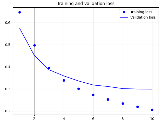
pyplot.plot(epochs, acc, 'bo', label='Training acc')
pyplot.plot(epochs, val_acc, 'b', label='Validation acc')
pyplot.title('Training and validation accuracy')
pyplot.legend()
pyplot.grid()
pyplot.subplots_adjust(left=0.08, right=0.98, top=0.94, bottom=0.06)
pyplot.show()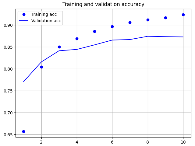
在上图中,点表示训练损失和准确度,实线表示验证损失和准确度。
请注意,在每个回合中,训练误差减少,训练准确率提高。这是使用梯度下降优化所期望的 -- 它在每个迭代中最小化损失。
但验证损失和准确率并非如此,它们似乎提前到达了峰值。这是一个过拟合的例子:模型在训练数据上的表现比在从未见过的数据上表现更好。
2.2.4.3 预测
要获得新示例的预测,将文本进行预处理后调用 Model.predict 函数即可:
examples = tf.constant([
    "The movie was great!",
    "The movie was okay.",
    "The movie was terrible..."
])
print(model.predict(vectorize_layer(examples)))
1/1 ━━━━━━━━━━━━━━━━━━━━ 0s 46ms/step
[0.44957402 0.2618876 0.18638325]
print(numpy.round(model.predict(vectorize_layer(text_batch)), 3).squeeze())
print(label_batch)
1/1 ━━━━━━━━━━━━━━━━━━━━ 0s 44ms/step
[0.384 0.044 0.072 0.003 0.003 0.188 0.819 0.002 0.995 0.046 0.671 0.113
0.421 0.001 0.957 0.002 0.046 0.036 0.595 0.912 0.658 0.971 0.621 0.002
0.006 0.085 0.009 0. 0.243 0.227 0.007 0.017]
tf.Tensor([0 0 0 0 0 0 1 0 1 0 1 0 0 0 1 0 0 0 1 1 1 1 0 0 0 0 0 0 0 1 0 0], shape=(32,), dtype=int32)