1.5 micrograd
一个微型的对标量值进行自动求导的引擎!
创建日期: 2025-04-03
在本教程中将构建一个微型“autograd”引擎(Automatic Gradient 的缩写),它实现反向传播算法。该算法在 1986 年 Rumelhart 等人的论文 Learning Internal Representations by Error Propagation 中被广泛用于训练神经网络。
文件 micrograd.py 中的代码是神经网络训练的核心,它使我们能够更新神经网络的参数,以使其在某些任务上表现得更好,例如自回归语言模型中的下一个单词预测。所有现代深度学习库(例如 PyTorch, Tensorflow, JAX 等)都使用完全相同的算法,只是这些库的优化程度更高,功能也更丰富。
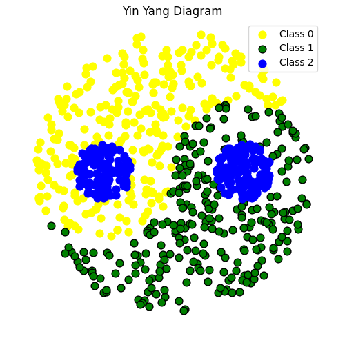
1.5.1 太极数据集
如下图所示,每个数据样本被归类为三种颜色类别之一,所有类别的样本数量大致相同:
1.5.2 Value 类型
Value 类用于表示标量值及其梯度,支持自动求导。它包含以下主要组件:
数据存储:
data用于存储标量值,grad 存储对应的梯度,初始为 0。反向传播:
_backward是一个方法,用于实现链式法则,在反向传播过程中更新梯度。操作记录:
_prev用于记录该值的前驱节点(即参与运算的操作数),_op存储产生该节点的操作名称(如加法、乘法等)。
class Value:
    """ stores a single scalar value and its gradient """

    def __init__(self, data, _prev=(), _op=''):
        self.data = data
        self.grad = 0
        # internal variables used for autograd graph construction
        self._backward = lambda: None
        self._prev = _prev
        self._op = _op # the op that produced this node, for graphviz / debugging / etc

    def __add__(self, other):
        other = other if isinstance(other, Value) else Value(other)
        out = Value(self.data + other.data, (self, other), '+')

        def _backward():
            self.grad += out.grad
            other.grad += out.grad
        out._backward = _backward

        return out

    def backward(self):

        # topological order all of the children in the graph
        topo = []
        visited = set()
        def build_topo(v):
            if v not in visited:
                visited.add(v)
                for child in v._prev:
                    build_topo(child)
                topo.append(v)
        build_topo(self)

        # go one variable at a time and apply the chain rule to get its gradient
        self.grad = 1
        for v in reversed(topo):
            v._backward()

    def __neg__(self): # -self
        return self * -1.0

    def __repr__(self):
        return f"Value(data={self.data}, grad={self.grad})"
支持的运算有加法、乘法、幂运算、ReLU、tanh、exp 和对数,每个操作会返回一个新的 Value 对象,并定义一个 _backward 方法来计算该操作的梯度。比如加法操作会将梯度累加到参与运算的两个 Value 对象上,乘法操作会按乘法法则更新梯度。
backward() 方法通过拓扑排序(按操作顺序)计算梯度,从输出节点开始,逐层向输入节点传播梯度,最终计算出每个变量的梯度。
这类实现了基本的自动微分功能,能帮助我们进行深度学习中常见的梯度计算。
1.5.3 构建神经网络
1.5.3.1 Module 基类
1.5.3.2 Neuron 类
1.5.3.3 Layer 类
1.5.3.4 MLP 多层感知机
将上面的结构体组合构建模型:
# init the model: 2D inputs, 8 neurons, 3 outputs (logits)
model = MLP(2, [8, 3])
1.5.4 训练
1.5.4.1 cross_entropy 损失
1.5.4.2 AdamW 优化器
1.5.4.3 训练过程
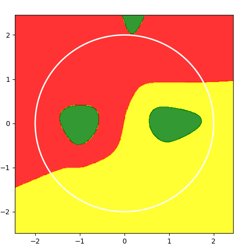
1.5.5 结果预测
def predict(model, x):
    x = (Value(x[0]), Value(x[1]))
    logits = model(x)
    label = numpy.argmax(numpy.array([v.data for v in logits]))
    return label
绘制边界函数:
def plot_decision_boundary(x, pred_func):
    # Set min and max values and give it some padding
    x_min, x_max = x[:, 0].min() - .5, x[:, 0].max() + .5
    y_min, y_max = x[:, 1].min() - .5, x[:, 1].max() + .5
    h = 0.01
    # Generate a grid of points with distance h between them
    xx, yy = numpy.meshgrid(numpy.arange(x_min, x_max, h),
                            numpy.arange(y_min, y_max, h))
    xx_ravel = xx.ravel()
    yy_ravel = yy.ravel()
    Z = []
    for x_coord, y_coord in zip(xx_ravel, yy_ravel):
        Z.append(pred_func(numpy.array([x_coord, y_coord])))
    Z = numpy.array(Z)
    Z = Z.reshape(xx.shape)
    pyplot.figure(figsize=(5, 5))
    pyplot.subplots_adjust(left=0.06, right=0.94, top=0.94, bottom=0.06)
    custom_cmap = ListedColormap(['red', 'yellow', 'green'])
    # Plot the contour and training examples
    pyplot.contourf(xx, yy, Z, cmap=custom_cmap, alpha=0.8)

    radius = 2.0  # Define the radius of the circle for decision boundary
    circle = pyplot.Circle((0, 0), radius, color='white',
                            fill=False, linewidth=2)
    pyplot.gca().add_artist(circle)
    pyplot.show()
预测结果: