6.1 Probability Theory
An overview of foundational probability and statistics concepts
Created Date: 2025-05-18
The core of this tutorial is to quickly help readers review the relevant knowledge of probability theory so as to better learn the diffusion model.
6.1.1 Normal Distribution
In probability theory and statistics, a normal distribution or Gaussian distribution is a type of continuous probability distribution for a real-valued random variable. The general form of its probability density function is:
The parameter \(\mu\) is the mean or expectation of the distribution (and also its median and mode), while the parameter \({\sigma}^2\) is the variance. The standard deviation of the distribution is \(\sigma\) (sigma). A random variable with a Gaussian distribution is said to be normally distributed, and is called a normal deviate.
The file normal_distribute.py sets \(\mu = 2\) and \(\sigma^2 = 10\), and uses NumPy to plot the normal distribution:
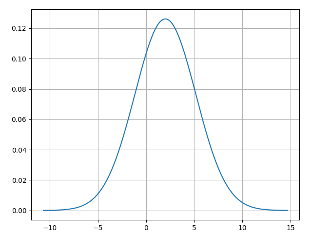
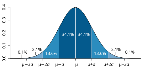
Image below illustrates a normal distribution curve, often referred to as a bell curve, showing how data is distributed around the mean (\(\mu\)) in a general normal distribution. The curve is symmetric with its peak at the mean \(\mu\), representing the highest probability density. The horizontal axis is labeled in units of standard deviation \(\sigma\), and the percentages indicate the proportion of data falling within each range:
The simplest case of a normal distribution is known as the standard normal distribution or unit normal distribution. This is a special case when \(\mu = 0\) and \({\sigma}^2 = 1\), and it is described by this probability density function (or density):
The normal distribution is often referred to as \(N(\mu, {\sigma}^2)\) or \(\mathcal{N}(\mu, \sigma^2)\). Thus when a random variable \(X\) is normally distributed with mean \(\mu\) and stanard deviation \(\sigma\), one may write:
6.1.1.1 Mean and Median
The mean is the sum of all values divided by the number of values. For numbers \(x_1, x_2, \cdots , x_n\):
The median is the middle number when the data is sorted.
If the number of data points is odd, the median is the middle value.
If even, it is the average of the two middle values.
6.1.1.2 Standard Deviation and Variance
Variance measures how spread out a set of numbers is. It's the average of the squared differences from the mean. You and your friends have just measured the heights of your dogs (in millimeters):
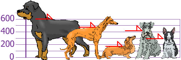
The heights (at the shoulders) are: 600 mm, 470 mm, 170 mm, 430 mm and 300 mm. Find out the Mean, the Variance, and the Standard Deviation.
Our first step is to find the Mean:
so the mean (average) height is 394 mm. Now we calculate each dog's difference from the Mean, let's plot this on the chart:
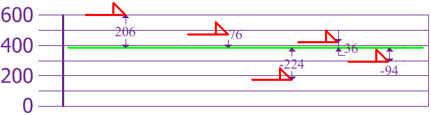
To calculate the Variance, take each difference, square it, and then average the result:
So the Variance is 21,704. And the Standard Deviation is just the square root of Variance, so:
And the good thing about the Standard Deviation is that it is useful. Now we can show which heights are within one Standard Deviation (147 mm) of the Mean:
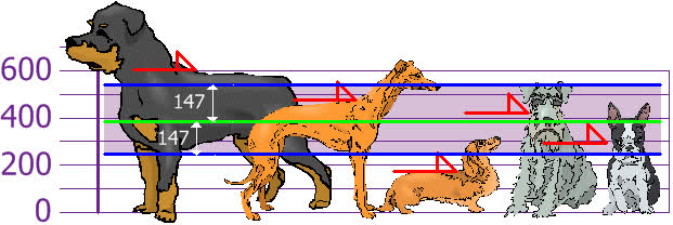
So, using the Standard Deviation we have a "standard" way of knowing what is normal, and what is extra large or extra small.
Rottweilers are tall dogs. And Dachshunds are a bit short, right?
Our example has been for a Population (the 5 dogs are the only dogs we are interested in). But if the data is a Sample (a selection taken from a bigger Population), then the calculation changes!
The Population: divide by \(N\) when calculating Variance (like we did)
A Sample: divide by \(N - 1\) when calculating Variance
The Population Standard Deviation:
The Sample Standard Deviation:
If our 5 dogs are just a sample of a bigger population of dogs, we divide by 4 instead of 5 like this:
\(Variance = \frac{108520}{4} = 27130\)
\(Deviation = \sqrt {27130} = 165\)
6.1.2 Covariance Matrix
Covariance is a statistical measure that tells us how two variables change together. In simpler terms, it indicates the direction of the linear relationship between two variables.
Here's a breakdown:
Positive Covariance: If the covariance is positive, it means that when one variable tends to be above its average, the other variable also tends to be above its average. Similarly, when one is below average, the other also tends to be below average. They move in the same direction.
Negative Covariance: If the covariance is negative, it means that when one variable tends to be above its average, the other variable tends to be below its average, and vice versa. They move in opposite directions.
Zero Covariance (or close to zero): If the covariance is zero or very close to zero, it suggests there's no linear relationship between the two variables. They tend to move independently of each other.
Covariance only tells you the direction of the relationship, not the strength. The magnitude of the covariance depends on the units of the variables, making it hard to compare covariances across different datasets. For strength, we use the correlation coefficient, which is a normalized version of covariance.
Simple Example: Study Hours and Test Scores
Let's say we want to see how the number of hours a student studies (Variable X) relates to their test score (Variable Y).
Here's some hypothetical data for 5 students:
| Student | Hours Studied (X) | Test Score (Y) |
|---|---|---|
| 1 | 2 | 60 |
| 2 | 4 | 75 |
| 3 | 6 | 85 |
| 4 | 8 | 90 |
| 5 | 5 | 70 |
Formula for sample convariance:
Where:
\(X_i\) is an individual ovservation of X.
\(Y_i\) is an individual ovservation of Y.
\(\bar X\) is the mean of X.
\(\bar Y\) is the mean of Y.
\(n\) is the number of observations.
Let's calculate step-by-step.
Step 1 - Calculate the means (\(\bar X\) and \(\bar Y\)):
\(\bar X = (2 + 4 + 6 + 8 + 5) / 5 = 5\)
\(\bar Y = (60 + 75 + 85 + 90 + 70) / 5 = 76\)
Step 2 - Calculate the deviations from the mean for each observation:
| Student | \(X_i\) | \(Y_i\) | \(X_i - \bar X\) | \(Y_i - \bar Y\) | \((X_i - \bar X)(Y_i - \bar Y)\) |
|---|---|---|---|---|---|
| 1 | 2 | 60 | (2 - 5) = -3 | (60 - 76) = - 16 | (-3) * (-16) = 48 |
| 2 | 4 | 75 | (4 - 5) = -1 | (75 - 76) = -1 | (-1) * (-1) = 1 |
| 3 | 6 | 85 | (6 - 5) = 1 | (85 - 76) = 9 | 1 * 9 = 9 |
| 4 | 8 | 90 | (8 - 5) = 3 | (90 - 76) = 14 | 3 * 14 = 42 |
| 5 | 5 | 70 | (5 - 5) = 0 | (70 - 76) = -6 | 0 * (-6) = 0 |
Step 3 - Sum the products of the deviations:
Step 4 - Divide by \(n - 1\), since we have 5 students:
6.1.3 Euler–Maruyama Method
The Euler–Maruyama method is a numerical method used to approximate the solution of a stochastic differential equation (SDE) . It is essentially an extension of the standard Euler method for ordinary differential equations (ODEs), modified to handle the random, noisy component of an SDE.
The method works by discretizing time into small steps and iteratively calculating the next value of the solution based on its current value. It approximates the continuous path of the SDE with a series of discrete jumps. The size of these jumps depends on both the deterministic drift and the stochastic diffusion terms of the SDE. For an SDE of the form:
\(Y_t\) is the stochastic process.
\(f(Y_t, t)\) is the drift term (deterministic part).
\(g(Y_t, t)\) is the diffusion term (stochastic part).
\(dW_t\) is the increment of a Wiener process (Brownian motion).
The Euler-Maruyama approximation is given by the iterative formula:
\(Y_i\) is the approximation of the solution at time \(t_i\).
\(\Delta t = t_{i+1} - t_{i}\) is the time step.
\(\Delta W_i = W_{t_{i+1}} - W_{t_i}\) is the Wiener process increment over the time step \(\Delta t\) , This increment is a random variable drawn from a normal distribution with mean 0 and variance \(\Delta{t}\) (i.e., \(\mathcal{N}(0, \Delta{t})\)).
The simulate_gbm function simulates a single path of a Geometric Brownian Motion (GBM) using the Euler-Maruyama method. This is a common way to model asset prices, as it incorporates both a deterministic growth trend and a stochastic (random) component.
def simulate_gbm(mu=0.1, sigma=0.2, s0=1.0, T=1.0, N=1000, seed=1):
    rng = numpy.random.default_rng(seed)
    dt = T / N
    sqrt_dt = numpy.sqrt(dt)
    t = numpy.linspace(0, T, N+1)
    S = numpy.empty(N+1)
    S[0] = s0
    for i in range(N):
        dW = sqrt_dt * rng.standard_normal()
        S[i+1] = S[i] + mu * S[i] * dt + sigma * S[i] * dW
    return t, S

t, S = simulate_gbm()
The code implements the discretized version of the GBM stochastic differential equation (SDE):
which is approximated by the Euler-Maruyama formula:
The returned arrays \(t, S\) can then be plotted to visualize the simulated path of the Geometric Brownian Motion
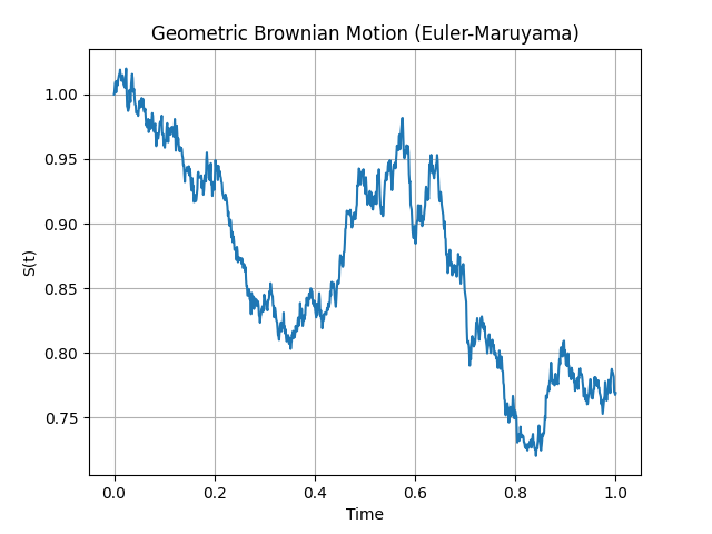
Figure 6 - Geometric Brownian Motion