DQN

10.4 DQN

Reinforcement Learning (DQN) Tutorial

Created Date: 2025-06-16

This tutorial shows how to use PyTorch to train a Deep Q Learning (DQN) agent on the CartPole-v1 task from Gymnasium. You might find it helpful to read the original Deep Q Learning (DQN) paper.

10.4.1 Task

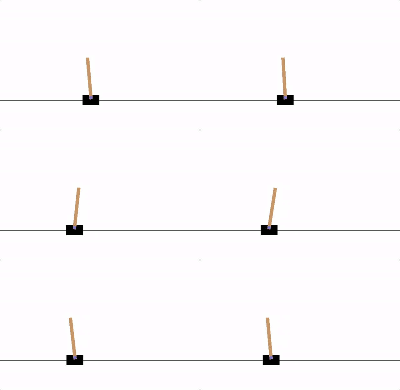
The agent has to decide between two actions - moving the cart left or right - so that the pole attached to it stays upright. You can find more information about the environment and other more challenging environments at Gymnasium’s website.

Figure 1 - Cart Pole

As the agent observes the current state of the environment and chooses an action, the environment transitions to a new state, and also returns a reward that indicates the consequences of the action. In this task, rewards are +1 for every incremental timestep and the environment terminates if the pole falls over too far or the cart moves more than 2.4 units away from center. This means better performing scenarios will run for longer duration, accumulating larger return.

The CartPole task is designed so that the inputs to the agent are 4 real values representing the environment state (position, velocity, etc.). We take these 4 inputs without any scaling and pass them through a small fully-connected network with 2 outputs, one for each action. The network is trained to predict the expected value for each action, given the input state. The action with the highest expected value is then chosen.

First, let’s import needed packages. Firstly, we need gymnasium for the environment, installed by using pip:

pip3 install gymnasium

10.3.2 Replay Memory

10.4.3 DQN Algorithm

Our environment is deterministic, so all equations presented here are also formulated deterministically for the sake of simplicity. In the reinforcement learning literature, they would also contain expectations over stochastic transitions in the environment.

Our aim will be to train a policy that tries to maximize the discounted, cumulative reward \(R_{t_0} = \sum_{t = t_0}^{\infty} {\gamma}^{t - t_0} \cdot r_t\), where \(R_{t_0}\) is also known as the return. The discount, \(\gamma\), should be a constant between 0 and 1 that ensures the sum converges. A lower \(\gamma\) makes rewards from the uncertain far future less important for our agent than the ones in the near future that it can be fairly confident about. It also encourages agents to collect reward closer in time than equivalent rewards that are temporally far away in the future.

The main idea behind Q-learning is that if we had a function \(Q^*: State \times Action \rightarrow \mathbb{R}\), that could tell us what our return would be, if we were to take an action in a given state, then we could easily construct a policy that maximizes our rewards:

\(\pi^*(s) = \arg\!\max_a \ Q^*(s, a)\)

However, we don’t know everything about the world, so we don’t have access to \(Q^*\). But, since neural networks are universal function approximators, we can simply create one and train it to resemble \(Q^*\).

For our training update rule, we’ll use a fact that every \(Q\) function for some policy obeys the Bellman equation:

\(Q^{\pi}(s, a) = r + \gamma Q^{\pi}(s', \pi(s'))\)

The difference between the two sides of the equality is known as the temporal difference error,:

\(\sigma = Q(s, a) - (r + \gamma \mathop{\max}\limits_{a}^{\prime} Q(s', a))\)

To minimize this error, we will use the Huber loss. The Huber loss acts like the mean squared error when the error is small, but like the mean absolute error when the error is large - this makes it more robust to outliers when the estimates of \(Q\) are very noisy. We calculate this over a batch of transitions, \(B\), sampled from the replay memory:

                    \(\mathcal{L} = \frac{1}{|B|} \sum_{(s, a, s', r) \ \in B} \mathcal{L}(\delta)\)
                

                    \[\text{where} \quad \mathcal{L}(\delta) = \begin{cases}
  \frac{1}{2}{\delta^2}  & \text{for } |\delta| \le 1, \\
  |\delta| - \frac{1}{2} & \text{otherwise.}
\end{cases}\]
                

Our model will be a feed forward neural network that takes in the difference between the current and previous screen patches. It has two outputs, representing \(Q(s, left)\) and \(Q(s, right)\) (where \(s\) is the input to the network). In effect, the network is trying to predict the expected return of taking each action given the current input.

10.4.4 Training

This cell instantiates our model and its optimizer, and defines some utilities:

select_action - will select an action according to an epsilon greedy policy. Simply put, we’ll sometimes use our model for choosing the action, and sometimes we’ll just sample one uniformly. The probability of choosing a random action will start at EPS_START and will decay exponentially towards EPS_END. EPS_DECAY controls the rate of the decay.

plot_durations - a helper for plotting the duration of episodes, along with an average over the last 100 episodes (the measure used in the official evaluations). The plot will be underneath the cell containing the main training loop, and will update after every episode.

Finally, the code for training our model.

Here, you can find an optimize_model function that performs a single step of the optimization. It first samples a batch, concatenates all the tensors into a single one, computes \(Q(s_t, a_t)\) and \(V(s_{t+1}) = {max}_a Q(s_{t+1}, a), and combines them into our loss. By definition we set \(V(s) = 0\) if \(s\) is a terminal state.

We also use a target network to compute \(V(s_{t+1})\) for added stability. The target network is updated at every step with a soft update controlled by the hyperparameter TAU, which was previously defined.

Below, you can find the main training loop. At the beginning we reset the environment and obtain the initial state Tensor. Then, we sample an action, execute it, observe the next state and the reward (always 1), and optimize our model once. When the episode ends (our model fails), we restart the loop.

Below, num_episodes is set to 600 if a GPU is available, otherwise 50 episodes are scheduled so training does not take too long. However, 50 episodes is insufficient for to observe good performance on CartPole. You should see the model constantly achieve 500 steps within 600 training episodes. Training RL agents can be a noisy process, so restarting training can produce better results if convergence is not observed.