1.5 Calculus
Calculus Volume 1 - OpenStax
Created Date: 2025-05-10
Just quickly familiarize yourself with the core concepts of calculus and recall the math classes you have taken. If you have not studied it, you need to read the recommended textbooks in detail.
1.4.1 Functions and Graphs
In this section, we provide a formal definition of a function and examine several ways in which functions are represented—namely, through tables, formulas, and graphs. We study formal notation and terms related to functions. We also define composition of functions and symmetry properties. Most of this material will be a review for you, but it serves as a handy reference to remind you of some of the algebraic techniques useful for working with functions.
1.4.1.1 Review of Functions
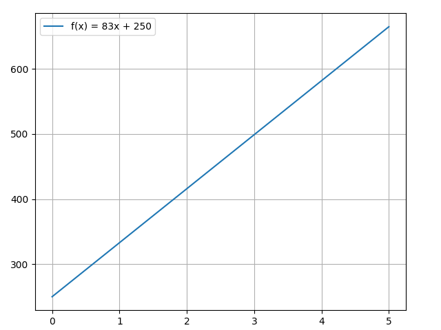
Linear functions have the form \(f(x) = ax + b\), where \(a\) and \(b\) are constants. The following figure plots \(f(x) = 83x + 250\):
Consider line \(L\) passing through points \((x_1, y_1)\) and \((x_2, y_2)\). Let \(\triangle{y} = y_2 - y_1\) and \(\triangle{x} = x_2 - x_1\) denote the changes in \(y\) and \(x\), respectively. The slope of the line is:
1.4.1.2 Basic Classes of Functions
A linear function is a special type of a more general class of functions: polynomials. A polynomial function is any function that can be written in the form:
for some integer \(n \ge 0\) and constants \(a_n, a_{n-1}, \cdots, a_0\), where \(a_n \ne 0\).
1.4.1.3 Trigonometric Functions
1.4.1.4 Inverse Functions
1.4.1.5 Exponential and Logarithic Functions
1.4.2 Limits
1.4.2.1 A Preview of Calculus
1.4.2.2 The Limit of a Function
1.4.2.3 The Limit Laws
1.4.2.4 Continuity
1.4.2.5 The Precise Definition of a Limit
1.4.3 Derivatives
1.4.3.1 Defining the Derivative
Now that we have both a conceptual understanding of a limit and the practical ability to compute limits, we have established the foundation for our study of calculus, the branch of mathematics in which we compute derivatives and integrals.
Tangent Lines
We begin our study of calculus by revisiting the notion of secant lines and tangent lines. Recall that we used the slope of a secant line to a function at a point \((a, f(a))\) to estimate the rate of change, or the rate at which one variable changes in relation to another variable. We can obtain the slope of the secant by choosing a value of \(x\) near \(a\) and drawing a line through the points \((a, f(a))\) and \((x, f(x))\). The slope of this line is given by an equation in the form of a difference quotient:
We can also calculate the slope of a secant line to a function at a value a by using this equation and replacing \(x\) with \(a + h\), where \(h\) is a value close to 0. We can then calculate the slope of the line through the points \((a, f(a))\) and \((a + h, f(a + h))\). In this case, we find the secant line has a slope given by the following difference quotient with increment \(h\):
These two expressions for calculating the slope of a secant line are illustrated in Figure 1. We will see that each of these two methods for finding the slope of a secant line is of value. Depending on the setting, we can choose one or the other. The primary consideration in our choice usually depends on ease of calculation.
The Derivative of a Function at a Point
1.4.3.2 The Derivative as a Function
Let \(f\) be a function. The derivative function, denoted by \(f'\) , is the function whose domain consists of those values of \(x\) such that the following limit exists:
1.4.3.3 Differentiation Rules
The Constant Rule
We first apply the limit definition of the derivative to find the derivative of the constant function, \(f(x) = c\) . For this function, both \(f(x) = c\) and \(f(x+h) = c\) , so we obtain the following result:
The rule for differentiating constant functions is called the constant rule. It states that the derivative of a constant function is zero; that is, since a constant function is a horizontal line, the slope, or the rate of change, of a constant function is 0. We restate this rule in the following theorem.
The Power Rule
Let \(n\) be a positive integer. If \(f(x) = x^n\) , then \(f'(x) = n x^{n-1}\) .
Alternatively, we may express this rule as \(\frac{d}{x} x^n = n x^{n-1}\)
The Sum, Difference, and Constant Multiple Rules
Let \(f(x)\) and \(g(x)\) be differentiable functions and \(k\) be a constant. Then each of the following equations holds.
Sum Rule. The derivative of the sum of a function \(f\) and a function \(g\) is the same as the sum of the derivative of \(f\) and the derivative of \(g\) .
Difference Rule. The derivative of the difference of a function \(f\) and a function \(g\) is the same as the difference of the derivative of \(f\) and the derivative of \(g\) :
Constant Multiple Rule. The derivative of a constant \(k\) multiplied by a function \(f\) is the same as the constant multiplied by the derivative:
1.4.3.4 Derivatives as Rates of Change
1.4.3.5 Derivatives of Trigonometric Functions
1.4.3.6 The Chain Rule
We have seen the techniques for differentiating basic functions (\(x^n\), \(sinx\), \(cosx\), etc.) as well as sums, differences, products, quotients, and constant multiples of these functions. However, these techniques do not allow us to differentiate compositions of functions, such as \(h(x) = sin(x^3)\) or \(k(x) = \sqrt{3x^2 + 1}\). In this section, we study the rule for finding the derivative of the composition of two or more functions.